The renormalization group on networks

Modern physics is actually one big quest to solve the many-body problem. Most often stated in soundbites invented by famous people from for example the influential Santa Fé school, but sometimes as old as Aristotle, such as “the whole is greater than the sum of the parts”. In physics this often came to mean: the whole is the sum of parts plus all their interactions. These interactions can sometimes be neatly organised in the form of Feynmann diagrams, the mysterious drawings you might sometimes see on the cover of physics books.

Blocks

Not exactly a new kid on the block, we are somewhere in the 50s-70s, group renormalization became a tool in particle physics to cope with the many possible interactions between elementary particles. First of all, the physicists borrowed from the old idea of considering a system at different scales. Think of the different resolutions of for example Google maps. Secondly, the physicist gave up on the idea that a system could be described by a finite number of interactions, but instead of that realised that an infinite number of interactions would not be such a big problem if the relation of the “interaction landscape” (my words) on one scale would have a simple reation with the “interaction landscape” on another scale. The example often used in statistical physics is that of the Ising model which is a 2D grid with so-called spins, that can point upwards or downwards. The spins influence their neighbours: a spin aligns its orientation according to the majority of its neighbours. By considering the larger scale of so-called block spins, we take blocks of say 3x3 spins and assign a spin direction to this larger block. Now, we have to come up with a description for the interactions between the block spins on this higher level. Not only that, but these interactions should also somehow be a coarse grained description of the interactions on the lower level. The idea of group renormalisation is that by repeating this pattern we end up with a flow from one “interaction landscape” to another: a flow through the space of coupling constants. We now miss one important piece of the puzzle to make sense of all this. This “flow” can namely be very chaotic. However, there is one specific phenomenon that is deeply related to the concept of scale invariance, which is the second order phase transition. A second order phase transition is a critical phenomenon that makes a system transition from one state to another in a very abrupt manner. Think earthquakes, crackling noise, etc. A system that is “poised at this edge of chaos” corresponds to a group renormalisation flow that is directed towards a fixed point! We suddenly have a way to describe the global behaviour - through a huge series of scales - from local interactions!

Network

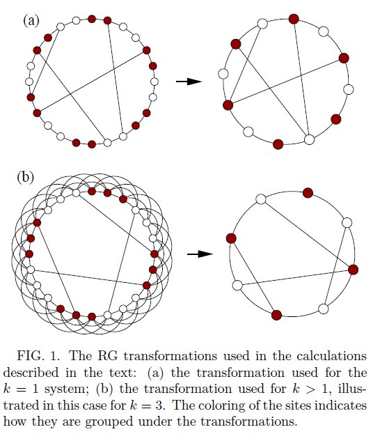
This is all very well, but nothing makes much sense without examples. We can give an example of the Ising model, or of self-organised criticality with sandpiles (Bak), but for swarm robotics, we are most interested in graphs. We have one remark here, most graph-based research disregards the spatial embedding of this graph in the real world, however, in our case of a network of robots, this is instead one of the most interesting and challenging future directions of “complex systems” research. The scientific world has been talking the last decade about networks with the so-called small world property. Imagine a network of people, where people correspond to the nodes on a graph and people that know each other are represented by edges. Imagine these nodes on a circle, and organise them a bit and you will see a structure as in Fig. 1 (from Newman and Watts publicly available paper [1]). The hypothesis is that this small world property is a critial phenomenon, and hence group renormalization can be applied.

Parameters L, k and p

We just summarize Newman and Watts findings here… The authors want to show that if the number of “shortcuts” goes to zero, the system exhibits a second- order phase transition observing the parameter $l$, the average distance between vertices. Besides the system size $L$, and a parameter $k$ which stands for some fixed range for which every node is connected to all its neighbours, there is a random parameter $p$. This $p$ stands for a rewiring probability for every $kL$ connection (and is “quenched”, that means, it is only done once). The renormalization procedure can be divided into two different cases, which is very typical for the procedure. For $k=1$, their blocking procedure takes two subsequent vertices on the ring and replaces them by one vertex. A “shortcut” to one of the vertices is preserved and will now point to the new vertex. The number of vertices $L$ becomes $L/2$. The number of edges goes from $L$ to $L/2$ and hence the probability to pick a given edge goes from $p$ to $2p$. For the case of $k>1$, the system size goes from $L$ to $L/k$, the probability from $p$ to $k^2 p$, the range parameter goes from $k$ to $1$, and the mean distance stays the same. Hence, every system with $k>1$ can be converted in a system with $k=1$ and then a group renormalisation procedure can be applied over and over again.

The transition

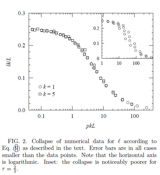
The authors write down an expression for $l$, the average distance between vertices. Let us not repeat the exact form of this equation, but explain between which regimes the mentioned transition would take place. If a system is really small, then for a given fixed $p$, there is on average less than one shortcut in the graph. This means that the average distance between vertices just happens over the ring and hence scales linearly with the system size $L$. However, when the system becomes larger, and $p$ is still fixed, in the end shortcuts will show up, and the distance between vertices will scale logarithmic with respect to $L$. The transition between these two regimes is the one that interests us.

Conclusion

In Fig. 2 you can see that the authors indeed were able to show this continous phase transition in the system. So, what do we have here!? We have a relation between system size and the famous average number of “degrees of separation” between nodes on a network. Now, you would be able to be all cocky on parties and tell fellow nerds that it’s not just six degrees of separation between you and some famous person, but that this depends on $L$, $p$ and $k$: the system size, the number of shortcuts, and the range of neighbours someone has.

This text introduced the renormalization group in networks. Interesting would be take these results and check how it can be applied to swarm robotics!

[1] Renormalization group analysis of the small-world network model, 2009, T. Payne